Outcome regression and propensity scores
What If: Chapter 15
Elena Dudukina
2021-12-08
1 / 13
Introduction
- Non-g(generalized) methods, e.g. outcome regression and propensity score-based methods don't work in a complex scenario with time-varying treatments
2 / 13
15.1 Outcome regression
Our causal contrast of interest:
- E[Ya=1,c=0]−E[Ya=0,c=0] or in words, the risk difference (average causal effect) under exposure level a=1 as compared with the same population under exposure level a=0 had no one been censored and in the absense of the sources of the systematic errors
Our assumptions:
- The exposed and non-exposed are exhangeable given confounders L:
- Ya⊥⊥A|L]
- Exposure consistency assumption, or the exposure variants are irrelevant (well-defined intervention)
- Positivity assumption (we observe exposed and unexposed in every level of every confounder)
- No interferance (the potential outcome in one participant is independent of the exposure level of another participant)
- The exposed and non-exposed are exhangeable given confounders L:
3 / 13
15.1 Outcome regression
G-methods: IPT weighting, standardization (parametric g-formula), g-estimation
Consider structural model:
- E[Ya,c=0|L]=β0+β1a+β2aL+β3L
- average causal effect of A on Y in each stratum of L is the function of β1 and β2
- the average causal effect of A on Y under no treatment (a=0) in each stratum of L is the function of β0 and β3
- suggesting that β3 is the causal effect of L is "table 2 fallacy"
Given all assumptions hold, we can estimate the desired contrast (parameters of the structural model) using outcome regression:
- E[Y|A,C=0,L]=α0+α1A+α2AL+α3L
- adjustment estimates causal effects in each stratum of L
- in unbiased situation, parameters β are the same as α are the same
- we computed conditional effect estimated (since we did not standardize over L as in g-formula or IPTW approaches)
4 / 13
15.1 Outcome regression
library(tidyverse)library(magrittr)# getting the datadata <- readr::read_csv(file = "https://cdn1.sph.harvard.edu/wp-content/uploads/sites/1268/1268/20/nhefs.csv") %>% mutate( education = case_when( education == 1 ~ "8th grade or less", education == 2 ~ "HS dropout", education == 3 ~ "HS", education == 4 ~ "College dropout", education == 5 ~ "College or more", T ~ "missing" ) ) %>% mutate(across(.cols = c(sex, race, education, exercise, active), .fns = forcats::as_factor)) %>% drop_na(qsmk, sex, race, education, exercise, active, wt82)# what's inside?data %>% select(qsmk, age, sex, race, education, wt71, smokeintensity, smokeyrs, exercise, active)## # A tibble: 1,566 x 10## qsmk age sex race education wt71 smokeintensity smokeyrs exercise## <dbl> <dbl> <fct> <fct> <fct> <dbl> <dbl> <dbl> <fct> ## 1 0 42 0 1 8th grade or ~ 79.0 30 29 2 ## 2 0 36 0 0 HS dropout 58.6 20 24 0 ## 3 0 56 1 1 HS dropout 56.8 20 26 2 ## 4 0 68 0 1 8th grade or ~ 59.4 3 53 2 ## 5 0 40 0 0 HS dropout 87.1 20 19 1 ## 6 0 43 1 1 HS dropout 99 10 21 1 ## 7 0 56 1 0 HS 63.0 20 39 1 ## 8 0 29 1 0 HS 58.7 2 9 2 ## 9 0 51 0 0 HS dropout 64.9 25 37 2 ## 10 0 43 0 0 HS dropout 62.3 20 25 2 ## # ... with 1,556 more rows, and 1 more variable: active <fct>5 / 13
Otcome regression
Fitting the model
# fit a regression of the outcome on the exposure and confoundersfit <- glm(data = data, formula = wt82_71 ~ qsmk + sex + race + age + I(age*age) + education + smokeintensity + I(smokeintensity*smokeintensity) + smokeyrs + I(smokeyrs*smokeyrs) + exercise + active + wt71 + I(wt71*wt71), family = gaussian())fit %>% broom::tidy(conf.int = T) %>% filter(term == "qsmk")## # A tibble: 1 x 7## term estimate std.error statistic p.value conf.low conf.high## <chr> <dbl> <dbl> <dbl> <dbl> <dbl> <dbl>## 1 qsmk 3.46 0.438 7.90 5.36e-15 2.60 4.32# Hernan: model without any product terms yielded the estimate 3.5 (95% confidence interval: 2.6, 4.3) kg.6 / 13
15.2 Propensity scores
When using IPT-weigting or g-estimation, we computed the exposure probability given the covariables Pr[A=1|L] at an individual level in the dataset
τ(L) is the propensity score
- τ(L) is a conditional probability of exposure given covariables
- τ(L) is close to 0 for those with low treatment probabaility and close to 1 among those with high probability of the exposure
- in the ideal randomized trial (with the randomization probability of 0.5), the τ(L) would be 0.5 for all individuals
- in an observational study the true τ(L) is unknown and needs to be estimated from the data
7 / 13
15.2 Propensity scores
- Estimating PS
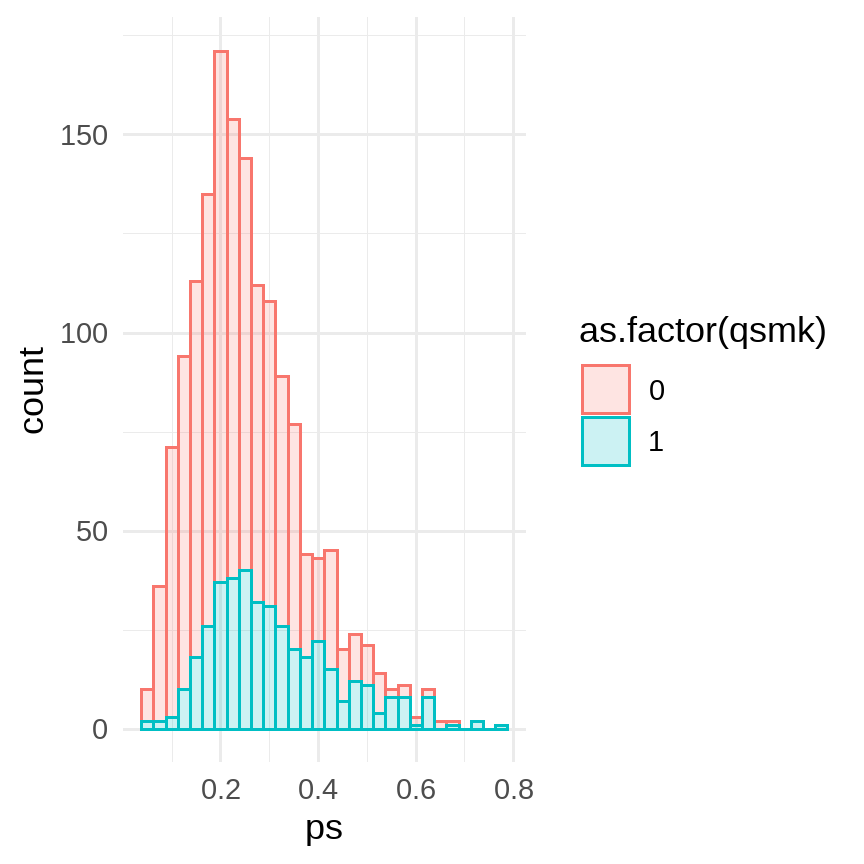
- PS histogram
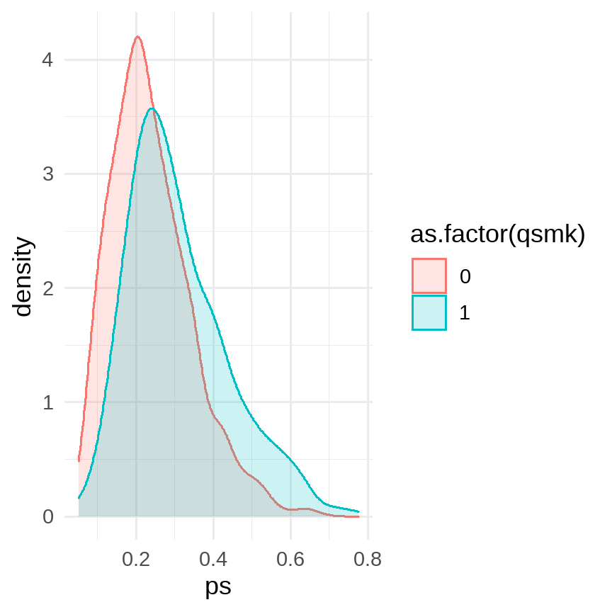
- PS density plot
- PS summary
- Fitting outcome regression model with PS as a covariable
- Outcome regression model with PS as a covariable
fit <- glm(qsmk ~ sex + race + age + I(age*age) + education + smokeintensity + I(smokeintensity*smokeintensity) + smokeyrs + I(smokeyrs*smokeyrs) + exercise + active + wt71 + I(wt71*wt71), data = data, family = binomial())data %<>% mutate( ps = predict(fit, type = "response", newdata = .))data %>% ggplot(aes(x = ps, color = as.factor(qsmk), fill = as.factor(qsmk))) + geom_histogram(alpha = 0.2, bins = 30) + # facet_grid(rows = vars(qsmk)) + theme_minimal(base_size = 12)
data %>% ggplot(aes(x = ps, color = as.factor(qsmk), fill = as.factor(qsmk))) + geom_density(alpha = 0.2) + # facet_grid(rows = vars(qsmk)) + theme_minimal(base_size = 12)
data %>% group_by(qsmk) %>% summarise(min = min(ps), mean = mean(ps), median = median(ps), max = max(ps))## # A tibble: 2 x 5## qsmk min mean median max## <dbl> <dbl> <dbl> <dbl> <dbl>## 1 0 0.0510 0.239 0.222 0.681## 2 1 0.0599 0.309 0.282 0.777fit <- glm(data = data, formula = wt82_71 ~ qsmk + ps) %>% broom::tidy(conf.int = T)fit %>% filter(term == "qsmk")## # A tibble: 1 x 7## term estimate std.error statistic p.value conf.low conf.high## <chr> <dbl> <dbl> <dbl> <dbl> <dbl> <dbl>## 1 qsmk 3.45 0.460 7.52 9.41e-14 2.55 4.35# Hernan: model without any product terms yielded the estimate 3.5 (95% confidence interval: 2.6, 4.3) kg.8 / 13
15.2 Propensity scores
- Smoking stoppers had higher PS than non-stoppers
- Individuals with the same propensity score values have different values of different covariables
- PS is a balancing score
- The of PS-based methods (IPTW, stratification, matching) still requires all causal assumptions (exchangeability given measured covariables, consistency, positivity, and no interference)
- Conditional exchangeability: Ya⊥⊥A=|L = Ya⊥⊥A=|τ(L)
- Positivity: no individual had a PS of 0 or 1
9 / 13
15.3 Propensity stratification and standardizaion
- Low chances that τ(L) will have the same value for two participants (continuous variable)
- Strata with similar although not the same values of τ(L) (eg deciles) --> potential lack of exchangeability between treated and untreated in some strata
- Fitting an outcome regression model with PS as a covariable
- Validity: causal assumptions and correct specification of the model Y ~ τ(L) (while IPTW is agnostic about this relation)
- Estimating the causal effect in each stratum and standardizing along the PS distribution to compute average causal effect
10 / 13
15.4 Propensity matching
- Under exchangeability and positivity given PS, associations in the matched population (matched pairs) are consistently estimating the associations in the whole population
- Exact matching is not effective
- Matching based on some value of closeness (s=0.05 or similar).
- If the closeness criterion is loose, the exchangeability between treated and untreated will be lost in the matched population
- If the closeness criterion is too tight, the exchangeability will hold but precision will be lost
- Unlike outcome regression with PS, the PS matching does not distinguish between random and structural non-positivity
- Matching may exclude treated with no matches among untreated --> initial and matched populations are not the same and the estimated effect is not average causal effect but average causal effect in the treated
- No clear view of who was excluded since propensity score value does not translate into patients characteristics straightforwardly
- Transportability of the effect measure computed for the matched population?
11 / 13
15.5 Propensity models, structural models, predictive models
- Aim of the study dictates what methods to use: causal or predictive
- Variable selection for answering causal questions is different from that when interested in a predictive task
12 / 13
References
- Hernán MA, Robins JM (2020). Causal Inference: What If. Boca Raton: Chapman & Hall/CRC (v. 30mar21)
13 / 13